

Machine Learning projects may seem complicated at first glance, but in reality, they follow a systematic flow that, once understood, makes the whole process quite straightforward. In this blog, we will provide a comprehensive guideline to help you navigate your machine learning projects smoothly.
Let's first sing a song to kickoff this blog
In a nutshell, what are we gonna talk about
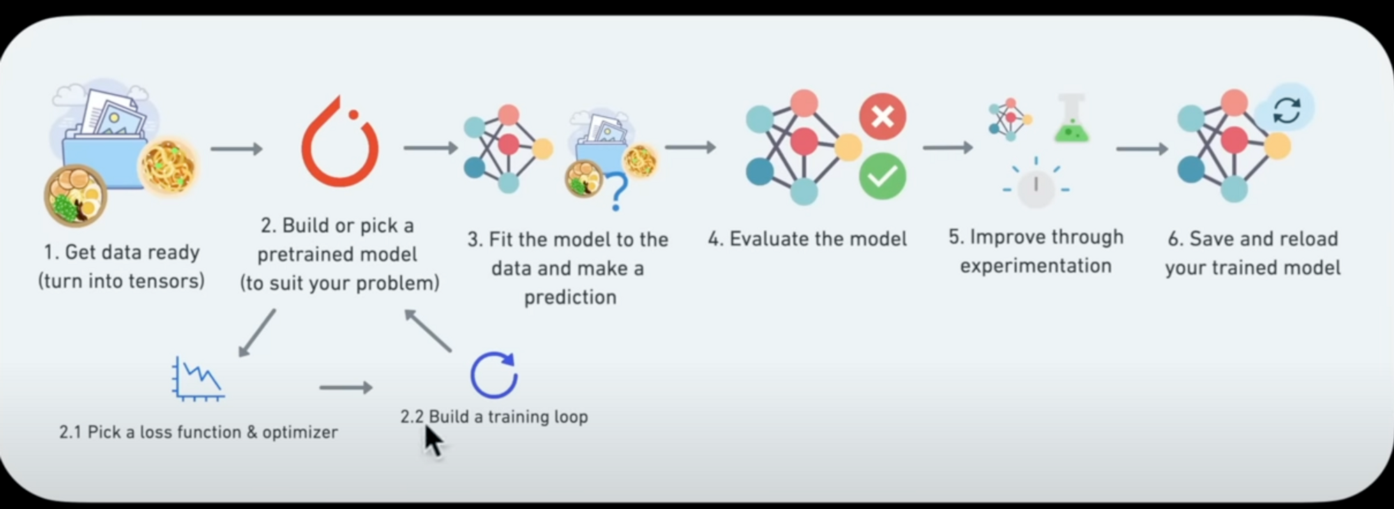
It's 6 basic steps - no matter what ML project or framework you're working with - it's usually always 6 steps. In this section, I'll be covering them in short but moving ahead, I'll share resources for templates and tricks for each step. Let's hear em out!
0. Become One with the Data
The initial step to every machine learning project is understanding your data. Make sure you visualise your data in as many ways as possible to gain insights. This could include checking the distribution of your data, identifying potential outliers, and understanding the relationship between different variables.
1. Preprocessing Your Data
Raw data is rarely ready for a machine learning model. You must preprocess your data to optimize it for learning. This may include tasks such as cleaning, normalization, and standardization of values.
When dealing with large datasets, it's common to divide them into smaller subsets known as "batches". A batch is a subset of the dataset that the model looks at while training. This is done because processing large datasets might not fit into the memory of your processor, and trying to learn patterns in the entire dataset in one go could result in the model not learning very well.
2. Creating a Model
Starting with a baseline model is an excellent approach for any machine learning project. A "baseline" is a relatively simple, existing model that you set up when you start your machine learning experiment. As you progress, you try to beat the baseline by experimenting with more complex or suitable models. Here you can explore the State of the Art algorithms to identify suitable models for your project.
3. Compiling and Fitting the Model
Once you have decided on your model, the next step is to compile it. This step involves defining the loss function, optimizer, and the evaluation metrics. After compiling, fit your model to the training data, allowing it to learn the underlying patterns.
4. Evaluating the Model
After your model has been fitted, it's time to evaluate its performance. Use your test data to evaluate how well the model generalizes to unseen data. This will give you an idea about how your model might perform in real-world scenarios.
5. Hyperparameter Tuning
In order to improve the model's performance, you will need to tune its hyperparameters. This process involves experimenting with various values for different hyperparameters to find the combination that provides the best performance.
Remember, overfitting and underfitting are two crucial aspects to consider during hyperparameter tuning. If your model is overfitting, consider using techniques such as data augmentation, regularization layers, or increasing your data. These techniques can help your model generalize better.
6. Iterate Until Satisfied
The above steps are not a one-time process. You might need to iterate over them several times before you achieve a satisfactory model performance. Keep experimenting until you have optimized your model.
8. Explore Advanced Techniques for Improvement
Once you have beaten your baseline, you can start exploring advanced techniques to further improve the performance of your model. This could involve adding more layers to your model, training for a longer period, finding an ideal learning rate, using more data, or using transfer learning.
Deep Diving into templates and tricks
Processing the Data
The first step in any machine learning project is to preprocess your data. Data augmentation and data shuffling are critical aspects of this stage.
Data augmentation is a technique used to increase the diversity of your data by making slight modifications to it, thereby enabling your model to learn more generalizable patterns. This technique is especially effective in image data, where actions such as rotating, flipping, and cropping an image can help diversify your dataset.
Shuffling data is essential to disrupt any inherent order that may exist in your dataset, such as all examples of a particular class clustered together. Shuffling ensures your model is exposed to various classes during training and avoids overfitting to a specific class. If your model displays erratic accuracy while training, consider shuffling your data.
When processing your data, you may consider various scaling techniques to standardize your dataset. For example:
- StandardScaler can give each feature zero-mean and unit standard deviation.
- MinMaxScaler provides a non-distorting, light-touch transformation.
- RobustScaler is useful for reducing the influence of outliers.
- Normalizer provides row-based normalization, using l1 or l2 normalization.
Refer to this cheat sheet for more information on preprocessing techniques.
Start with a Baseline
Starting with a simple baseline model allows us to have a reference point for comparing the improvements gained from enhancing our model. Fitting a baseline model typically involves three steps:
- Creating a model: Define the input, output, and hidden layers of a deep learning model.
- Compiling a model: Define the loss function, optimizer, and evaluation metrics for the model.
- Fitting a model: Train the model to find patterns between features and labels.
Baseline models can be created using various libraries such as PyTorch and TensorFlow, based on your project's requirements.
PyTorch
torch.manual_seed(42)

# Set the number of epochs (how many times the model will pass over the training data)
epochs = 100

# Create empty loss lists to track values
train_loss_values = []
test_loss_values = []
epoch_count = []

# Put data on the available device
# Without this, error will happen (not all model/data on device)
X_train = X_train.to(device)
X_test = X_test.to(device)
y_train = y_train.to(device)
y_test = y_test.to(device)

for epoch in range(epochs):
    ### Training

    # Put model in training mode (this is the default state of a model)
    model_0.train()

    # 1. Forward pass on train data using the forward() method inside
    y_pred = model_0(X_train)
    # print(y_pred)

    # 2. Calculate the loss (how different are our models predictions to the ground truth)
    loss = loss_fn(y_pred, y_train)

    # 3. Zero grad of the optimizer
    optimizer.zero_grad()

    # 4. Loss backwards
    loss.backward()

    # 5. Progress the optimizer
    optimizer.step()

    ### Testing

    # Put the model in evaluation mode
    model_0.eval()

    with torch.inference_mode():
      # 1. Forward pass on test data
      test_pred = model_0(X_test)

      # 2. Caculate loss on test data
      test_loss = loss_fn(test_pred, y_test.type(torch.float)) # predictions come in torch.float datatype, so comparisons need to be done with tensors of the same type

      # Print out what's happening
      if epoch % 10 == 0:
            epoch_count.append(epoch)
            train_loss_values.append(loss.detach().numpy())
            test_loss_values.append(test_loss.detach().numpy())
            print(f"Epoch: {epoch} | MAE Train Loss: {loss} | MAE Test Loss: {test_loss} ")
Tensorflow
# Now our data is normalized, let's build a model to find pattern

# Set a random seed
tf.random.set_seed(42)

# 1. Create a model
model_2 = tf.keras.Sequential([
    tf.keras.layers.Flatten(input_shape=(28,28)),
    tf.keras.layers.Dense(4, activation="relu"),
    tf.keras.layers.Dense(4, activation="relu"),
    tf.keras.layers.Dense(10, activation="softmax"),
])

# 2. Compile the model
model_2.compile(
    loss=tf.keras.losses.SparseCategoricalCrossentropy(),
    optimizer=tf.keras.optimizers.Adam(),
    metrics=["accuracy"]
)

# 3. Train the model
norm_history = model_2.fit(
    train_data_norm,
    train_labels,
    epochs = 10,
    validation_data = (
        test_data_norm,
        test_labels
    )
)
Plotting training and testing loss
## Plotting training and test loss

# Plot the loss curves
plt.plot(epoch_count, train_loss_values, label="Train loss")
plt.plot(epoch_count, test_loss_values, label="Test loss")
plt.title("Training and test loss curves")
plt.ylabel("Loss")
plt.xlabel("Epochs")
plt.legend();
Evaluating Our Model
Visualizing our model's predictions and its performance metrics is an integral part of model evaluation. Plots comparing ground truth labels and model predictions can provide insights into how well our model is performing. For regression problems, evaluation metrics like Mean Average Error (MAE) and Mean Squared Error (MSE) can be used to quantify the average errors of our model's predictions.
Tracking Experiments
Visualizing our model's predictions
Apart from that, a good way to proceed is visualize, visualize, visualize!
It's a good idea to visualize
- The data - What data are we working with? What does the data look like?
- The model itself - what does our model look like
- The training of a model - How does a model perform as it is learning?
- The predictions of the model -How do the predictions match up against the ground truth (the original labels)
To visualize our model's predictions, it's a good idea to plot them against ground truth values
def plot_predictions(train_data=X_train,
                     train_labels=y_train,
                     test_data=X_test,
                     test_labels=y_test,
                     predictions=None):
  """
  Plots training data, test data and compares predictions.
  """
  plt.figure(figsize=(10, 7))

  # Plot training data in blue
  plt.scatter(train_data, train_labels, c="b", s=4, label="Training data")

  # Plot test data in green
  plt.scatter(test_data, test_labels, c="g", s=4, label="Testing data")

  if predictions is not None:
    # Plot the predictions in red (predictions were made on the test data)
    plt.scatter(test_data, predictions, c="r", s=4, label="Predictions")

  # Show the legend
  plt.legend(prop={"size": 14});
To efficiently compare the performance of different models and configurations, it is essential to track the results of your experiments. Tools like TensorBoard and Weights & Biases can be useful in managing and visualizing your experiments' results.
Improving Our Model
Build the model -> fit it -> evaluate it -> tweak it -> fit it -> evaluate it -> tweak it -> ....
Improving model accuracy is an iterative process that involves revisiting the model creation, compilation, and training stages.
During the model creation stage, you might add more layers, increase the number of hidden units in each layer, or change the activation function. In the compilation stage, changing the optimization function or adjusting the learning rate could improve model performance. The training stage could involve training the model for more epochs or using a larger dataset.
This process of modifying various parameters to enhance the model's performance is known as "hyperparameter tuning".
Approaches to improve accuracy
- Get more data -> Get a larger dataset that we can train our model on
- Hyperparameter tuning -> Use more hidden layers or increase number of neurons in each hidden layer
- Train for longer -> Give your model more of a chance to find patterns in the dataset
Save a Model
Saving a model is essential for using it outside the training environment, like in a web or mobile application. Models can be stored in the SavedModel Format or the HDF5 Format in TensorFlow, depending on whether you plan to tweak and train the model further in TensorFlow or outside TensorFlow. In PyTorch, the recommended method is saving and loading the model's state_dict().
PyTorch code
from pathlib import Path

# 1. Create models directory
MODEL_PATH = Path("models")
MODEL_PATH.mkdir(parents=True, exist_ok=True)

# 2. Create model save path
MODEL_NAME = "01_pytorch_workflow_model_0.pth"
MODEL_SAVE_PATH = MODEL_PATH / MODEL_NAME

# 3. Save the model state dict
print(f"Saving model to: {MODEL_SAVE_PATH}")
torch.save(obj=model_0.state_dict(), # only saving the state_dict() only saves the models learned parameters
           f=MODEL_SAVE_PATH)
Run on GPU
Running your model on a GPU can significantly speed up training. You can check if your model is set to run on a GPU using the model.parameters().device function and set it to GPU using the model.to(device) function, where device is set to "cuda" for GPU or "cpu" for the Central Processing Unit.
Conclusion
In conclusion, understanding these steps will assist you in structuring your ML projects effectively. Remember, machine learning is an iterative process, and it's okay to go back and forth between steps to improve your model's performance.